
Uplift models are used to identify customers who are most likely to respond positively as a result of receiving some intervention. Some examples include customer retention campaigns, social welfare programs, etc. This post details some examples of uplift models in action.
Uplift modeling [1],[2] refers to models that predict the incremental change in behaviour caused by an intervention. While these models are commonly associated with marketing applications, they are just as relevant in any field where the task is to target specific segments of a population to maximise some benefit (e.g. education, social welfare, public health). Instead of focussing on an output variable (e.g. sales), uplift modeling focusses on the change in the output variable caused by an intervention (e.g. change in sales caused by email advertising).
As an example, consider a marketing campaign where customers are sent offers in order to persuade them to purchase a product. In this example, there is a binary treatment (i.e. the customer can either receive the offer or not) and a binary objective (i.e. the customer can either purchase or not). The uplift is the probability of purchasing (if they receive the offer) minus the probability of purchasing (if they do not receive the offer). This difference in probabilities is important, because the goal of uplift modeling in such a campaign is to avoid sending offers to customers who would have purchased it anyway.
A similar situation occurs in retention [3]. Consider a retention campaign where customers are selected to be contacted by a retention team to persuade them to continue their subscription. The goal is to only contact customers who can be persuaded to stay. We want to avoid contacting customers who always intended to stay or leave, regardless of being contacted. More importantly, we want to avoid contacting customers who may actually be prompted to leave because we have contacted them (e.g. it could prompt them to shop around for a better deal when they otherwise might not have).
The fundamental problem that uplift modeling solves is that a customer may either receive or not receive an intervention, they cannot do both. In a marketing campaign, they can either be in the treatment group or the control group, they cannot be in both. This means that the uplift of an individual customer cannot be measured directly, it can only be estimated based on groups of similar customers. Specifically, uplift is the conversion rate of customers in the treatment group minus the conversion rate of customers in the control group.
This definition helps us define four subgroups in a population:
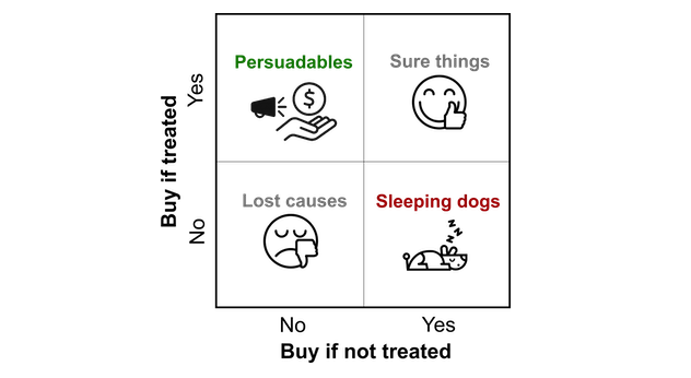
- Sure things (or always-takers) are customers who were always going to buy the product, regardless of whether or not they received a marketing intervention (zero uplift).
- Persuadables (or compliers) are customers who became more likely to buy the product because they received a marketing intervention (positive uplift).
- Sleeping dogs (or defiers) are customers who became less likely to buy the product because they received a marketing intervention (negative uplift).
- Lost causes (or never-takers) are customers who were never going to buy the product, regardless of whether or not they recieved a marketing intervention (zero uplift).
The premise behind uplift modeling is that it only makes sense to send marketing interventions to persuadables, because they are the only group where targeting them gives a better outcome than not targeting them. Sending marketing interventions to customers who are sure things or lost causes is a waste of resources, and an opportunity cost if you are constrained by the number of interventions you can send. Worse still, sending them to sleeping dogs will actually decrease sales.
It is important to distinguish uplift modeling from other types of modeling. Penetration (look-alike) models[4] characterise customers who have exhibited some particular behaviour (e.g. bought the product, churned). This assumption is that if we can find customers who haven’t shown this behaviour, but have similar attributes to customers who have, then they will be good targets for campaigns that prompt the behaviour (eg. cross-sell, retention). The flaw with this argument is that there may still be good reasons for not targeting the customer in this way. For example, they have already bought something similar from a competitor, or contacting may actually trigger them to churn.
Uplift modeling is also different to so-called ‘response’ modeling[5]. These models characterise customers who have exhibited a particular behaviour in apparent response to some direct marketing intervention. However, this type of model fails to consider the counterfactual case (i.e. how many customers would have bought it if there was no marketing invervention?). There may be customers who would have bought the product regardless of the marketing intervention. There may even be customers who intended to buy the product, but were put off by the direct marketing and decided not to buy the product.
Uplift data
Here, we will demonstrate some examples of uplift models using a publicly available dataset of simulated customers[6].
This dataset contains 10,000 customers and 19 context features. There is a binary treatment condition (treatment or control), and the customers are randomly and evenly split between the two:
{.table}
| Treatment or control | Number | Proportion |
|---|---|---|
| control | 5063 | 0.506 |
| treatment | 4937 | 0.494 |
There also a binary reward, positive or negative, which indicates each customer’s outcome after their assigned treatment:
{.table}
| Outcome | Number | Proportion |
|---|---|---|
| negative | 5047 | 0.505 |
| positive | 4953 | 0.495 |
Since this data has been simulated, the ‘ground truth’ of each customer’s type is known. Note that in real applications, we cannot know the ground truth of each customer, because that would require them to be assigned treatment and control simultaneously. In this example, the four customer types are evenly represented:
{.table}
| Customer type | Number | Proportion |
|---|---|---|
| lost_cause | 2554 | 0.255 |
| persuadable | 2471 | 0.247 |
| sleeping_dog | 2528 | 0.253 |
| sure_thing | 2447 | 0.245 |
Note that in real world data, we will not know what each customer’s type is, this is what uplift modeling is supposed to discover.
This dataset effectively simulates an A/B test, and we can calculate the uplift by subtracting the control conversion rate (0.496) from the target conversion rate (0.494), to give an overall uplift of -0.002. This shows that the overall effect of this offer on the population is negative.
However, if we calculate the treatment/control conversion rates and uplifts for each customer type separately, we see how they behave differently:
{.table}
| Customer type | Conversion rate (treatment) | Conversion rate (control) | Uplift |
|---|---|---|---|
| sure_thing | 1 | 1 | 0 |
| lost_cause | 0 | 0 | 0 |
| persuadable | 1 | 0 | 1 |
| sleeping_dog | 0 | 1 | -1 |
The ‘sure things’ and ‘lost causes’ both have zero uplift, because their target and control conversion rates are the same (100% for ‘sure things’, and 0% for ‘lost causes’). There is no benefit in applying treatment to these customers. For ‘persuadables’, however, there is 100% uplift, because the treatment conversion rate is 100%, while the control conversion rate is 0%. These are the customers that should be targeted for treatment. Conversely, the ‘sleeping dogs’ have a -100% uplift, which means that targeting these customers for treatment will drive them away from buying. These customers should not be contacted.
Let’s assume that we a running a campaign on this population, where it costs $1 to target each customer, and each successful conversion has $10 revenue. What would happen if we didn’t apply the treatment to any customers, or if we applied it to all of them? Also, what would happen if we only targeted persuadable customers for treatment?
The table below summarises what the results of such campaigns would be. Firstly, if we didn’t apply any treatment, then the cost of treatment would be zero. The conversions would come from the ‘sure things’ (who convert anyway) and the ‘sleeping dogs’ (who converted because we didn’t target them for treatment), resulting in a profit of $49,750. If we targeted all customers for treatment instead, we would have to include the cost of targeting them all. The ‘sure things’ would still convert, and so would the ‘persuadables’ (who only convert because we applied the treatment to them). However, we would also drive away the ‘sleeping dogs’ (they don’t convert because we applied treatment to them). This would result in a profit of $13,900. Finally, consider the case where we only apply the treatment to ‘persuadables’. The cost of treatment is reduced, because it only applies to a subset of the population. We also get the conversions from the ‘sure things’, ‘persuadables’, and ‘sleeping dogs’, giving a much higher profit of profit of $71,989.
{.table}
| Scenario | Cost | Revenue | Profit |
|---|---|---|---|
| Don’t apply any treatment | 0 | 49750 | 49750 |
| Apply treatment to all customers | 10000 | 23900 | 13900 |
| Apply treatment to persuadable customers only | 2471 | 74460 | 71989 |
Clearly, the best scenario is to apply the treatment to persuadable customers only. However, real campaigns will not be able to tell the type of each customer, which is why uplift modeling is used to estimate this.
Data collection practicalities
The data used in this example is synthetic, but real world data is unlikely to be as straightforward as this. For example, poor data quality can lead to direct mail interventions being sent to the wrong address, and even if they are sent to the right address, the customer may not read it. Email campaigns allow tracking of customers who open emails, but even this does not guarantee that they’ve read it. Customers may respond to interventions with different lag times, so there needs to be a fixed time window to determine how long you wait for them to respond after the intervention is sent.
Uplift models
Here, we will compare a benchmark oracle model with two uplift models, which are based on different approaches. These approaches were chosen because their implementations are simple to use, while still managing to model uplift directly.
Oracle
When evaluating uplift models, it is useful to compare them against benchmarks. A lower bound can be set by a uniform random assignment policy. This is the uplift a campaign would achieve if offers were sent to customers randomly. Our minimum expectation is that any useful uplift model must outperform this lower bound.
To define the upper bound, we can use the synthetically generated ground truth customer type (i.e. persuadables, sleeping dogs, etc.) to simulate how an all-knowing oracle model would perform. This oracle would only target persuadables for treatment, and would not target any other type of customer. This is the best performance that any uplift model can achieve, and we can evaluate uplift models according to how close they come to achieving this ideal performance.
Using the oracle, the predicted uplift is 100% for all persuadables, -100% for all sleeping dogs, and 0% for sure things and lost causes.
Causal Conditional Inference Forest
The first model we consider is the causal conditional inference forest
(CCIF)[7], which is based on binary decision trees. At each node in
the tree, it tests whether there is any interaction effect between the
treatment and the features. If any of them show an effect, then a
split is made using the feature showing the strongest effect. The
benefits of this approach are that it is less prone to overfitting, and
less biased towards selecting features with many possible splits (which
is common in tree-based approaches). The implementation used here comes
from the uplift[8] R package.
Transformed Outcome Tree
The second model we consider is the transformed outcome tree (TOT)[9],
which uses the treatment and outcome labels to create a new transformed
outcome. This transformed outcome is constructed such that its average
value corresponds to the average uplift. The benefit of this approach is
that once the simple transformation is done, the uplift problem becomes
a binary classification problem, and any of the standard machine
learning algorithms can be applied. The implementation used here comes
from the pylift[10] python package.
For the CCIF and TOT models, the dataset was partitioned into a 70:30 train:test split. The models were trained on the training data, and the evaluation on the test data is shown below.
Evaluating uplift models
Uplift by decile
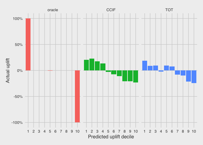
A simple way to evaluate uplift models is to compare their predicted uplift with their actual uplift. The uplift models generate a predicted uplift value for each customer. However, since actual uplift cannot be calculated for each individual customer (i.e. they cannot receive and not receive the offer simultaneously), we calculate the actual uplift over a group of customers. To do this, we rank the customers in the test dataset according to their predicted uplift, and partition them into deciles. The plots below show the actual uplift versus the predicted uplift deciles.
Because of the artificial nature of the oracle, its decile partitioning needs be rescaled due to ties (i.e. many customers have the same predicted uplift value). However, we see here that the top ‘decile’ has an actual uplift of 100%, since it contains all the persuadables. The bottom ‘decile’ has an actual uplift of -100%, since it contains all the sleeping dogs. The remaining sure things and lost causes have 0% uplift in the middle decile.
We see a more realistic trend for the CCIF model, where the top four deciles show positive uplift, and the bottom six deciles show negative uplift. The general trend is decreasing uplift from top to bottom deciles. From this plot, we would conclude that it only makes sense to target the top four deciles for treatment according to this model, as these are the only customers who show positive uplift.
We see a similar trend for the TOT model, where there is also a general trend is decreasing uplift from top to bottom deciles. However, the behaviour is not as consistent as in the CCIF model, because the fourth decile shows negative uplift, while the fifth and sixth deciles show positive uplift.
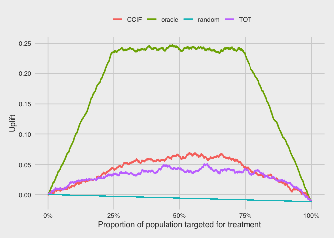
Qini curve
The uplift by decile plots above are useful for understanding how the uplift models are performing, but they make it harder to compare models to each other directly. Such comparisons are usually done using the qini curve [11] [12], which plots the cumulative uplift across the population. Here, we rank the customers by their predicted uplift on the horizontal axis, and the vertical axis plots the cumulative number of purchases in the treatment group (scaled by the total treatment size) minus the cumulative number of purchases in control (scaled by the total control size).
The straight line corresponds to randomly targeting customers for treatment. As more customers are targeted for treatment, the uplift decreases linearly to a final value of -0.01. This means that the overall effect of treatment all customers in this test dataset population is negative.
For the oracle, this curve increases sharply as the proportion of the population targeted for treatment increases from 0%. This is because the targeted customers are all persuadables, and they all contribute positive uplift. Once this population of persuadables is exhausted (at about 25%), the next customers to be targeted for treatment are all sure things and lost causes. These customers do not contribute any uplift, so the curve stays flat as this middle 50% (from 25% to 75%) gets targeted. Once this segment of the population is exhausted, the only customers left are the sleeping dogs, which contribute negative uplift. Continuing to apply treatment to these customers would reverse the uplift gains, until it reaches the final value of -0.01 from applying treatment to all customers.
For the CCIF and TOT uplift models, we see that they perform better than random, but worse than the oracle (as expected). The CCIF model appears to perform slightly better than the TOT model, since their uplift gains peak at approximately 0.07 and 0.05, respectively.
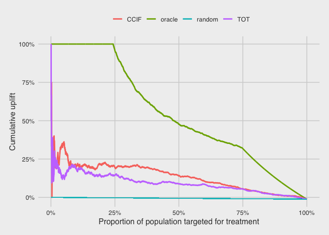
Cumulative uplift
Another way to compare the models is to plot their cumulative uplifts. Again, we rank the customers by their predicted uplift on the horizontal axis. The vertical axis plots the cumulative number of purchases in treatment (scaled by the cumulative treatment size) minus the cumulative number of purchases in control (scaled by the cumulative control size).
For the oracle, the uplift is consistently 100% for the first 25% of customers, because they are all persuadables. The uplift the decreases as there are no more purchases from the rest of the population.
For the CCIF and TOT models, the curves start off noisy due to the small size of the cumulative population here, but they settle to approximately 0.19 and 0.14 for CCIF and TOT, respectively, at the population proportion of 25%. Again, we see the CCIF model slightly outperforming the TOT model for this particular dataset.
Conclusion
If this was a real campaign (without the oracle), then we could reasonably use the CCIF model to rank customers by their predicted uplift and only target the top 20-40% for treatment, as these are the customers that we expect to be the most persuadable. We would expect the uplift from this campaign to be approximately 20%, which is much higher than the -1% uplift from applying the treatment to all customers.
The synthetic dataset in this example was designed to showcase the strengths of uplift modeling, and it reflects circumstances where uplift modeling is more effective:
- It has a large control group (equal in size to the treatment group). This is important because uplift is defined as the difference between treatment and control.
- There is a significant proportion of sleeping dogs. When there are customer who will respond negatively to treatment, it is important to avoid targeting them.
- There is some finite resource to be allocated. If the cost of treatment is high, then it becomes more important to only apply the treatment to customers where the predicted uplift is high.
- The features are informative of uplift, allowing effective uplift models to be built. Note that uplift is usually a much smaller effect to predict than overall conversion rate, so it is more difficult to predict. Also, the features that are predictive of overall conversion rate may not be predictive of uplift.
Uplift models built on datasets with these attributes are more likely to show effective results beyond conventional models.